In this tutorial, a dynamical decoupling sequence is applied to the electron spin of \(^{15}\)NV and used to obtain gates to the nuclear spin. We begin defining the NV system, following that we simulate the XY\(N\) spectra of the electron observable and compare them with simulations. Finally, we also simulate the behaviour of the nuclear spin. This notebook closely follows the work from:

• 12. Tsunaki, M. Dotan, K. Volkova, & B. Naydenov. (2025). Multi-Qubit Gates by Dynamical Decoupling Implemented with IBMQ and 15NV Center in Diamond. arXiv:2509.22107 quant-ph.

As this is a quite complex problem, physics discussions will be kept to a minimum here in favor of a focus to the simulation. For a detailed explanation of the problem, please refer to the original paper.

import numpy as np
import matplotlib.pyplot as plt
from scipy.stats import linregress
from qutip import qeye, jmat, tensor, fock_dm

from quaccatoo import NV, XY, ExpData

1. Definition of the NV System

We begin defining the NV system and the experimental conditions for the XY\(N\) pulse sequences.

system = NV(
    B0 = 32,
    theta = 2.9,
    units_angles = 'deg',
    units_B0 = 'mT',
    N=15
)

# experimental value of pi-pulse duration
t_pi = 0.025694/2
w1 = 1/t_pi/2

# number of pulses
N = np.arange(2, 30, 2)

# free evolution times
tau = np.arange(0.260, .260 + 50*0.004, 0.004)

2. Electron Spin

Now the simulations can be run in a loop over the N values and saved into a results array.

XYN_S_sim = np.empty(N.size, dtype=XY)

for idx in range(N.size):

    # defines the simulation object with the parameters
    XYN_S_sim[idx] = XY(
        free_duration = tau,
        pi_pulse_duration = t_pi,
        system = system,
        h1 = w1*system.MW_h1,
        pulse_params = {'f_pulse': system.MW_freqs[0]},
        M = int(N[idx]/2),
    )

    # runs the simulation and stores the results
    XYN_S_sim[idx].run()

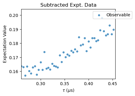
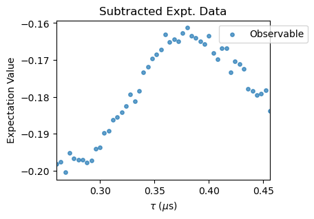
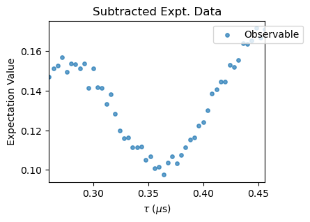
To compare these simulations with the experimental data, we load them with the ExpData class, convert the units of the pulse separation to us and subtract the columns 1 and 2 with the subtract_results_columns method to obtain the fluorescence as simulated. The experimental data was obtained and saved within Qudi software’s format.

XYN_exp = np.empty(N.size, dtype=ExpData)

for idx in range(N.size):
    XYN_exp[idx] = ExpData(f'./exp_data_tutorials/08/XY{N[idx]}.dat', results_columns=[1,2], variable_name=r'$\tau$ ($\mu$s)')

    # converts the time units to us
    XYN_exp[idx].variable *= 1e6

    XYN_exp[idx].subtract_results_columns(plot=True, figsize=(4,3))

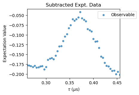
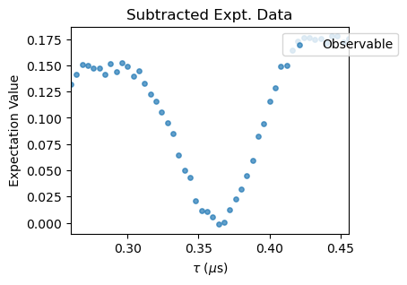
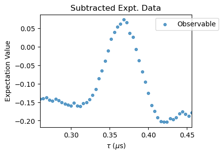
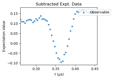
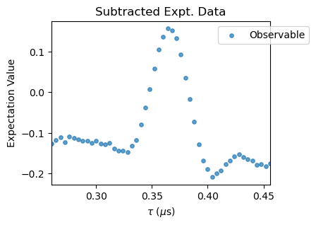
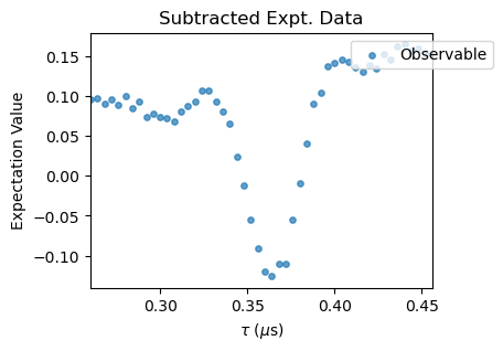
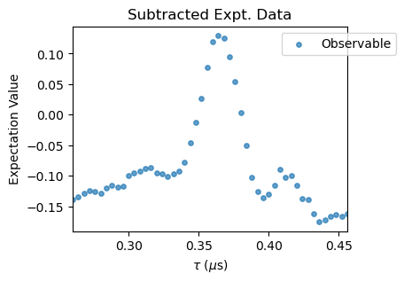
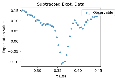
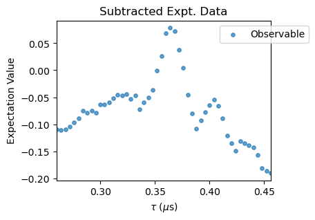
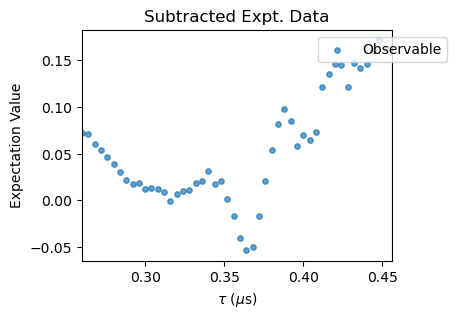
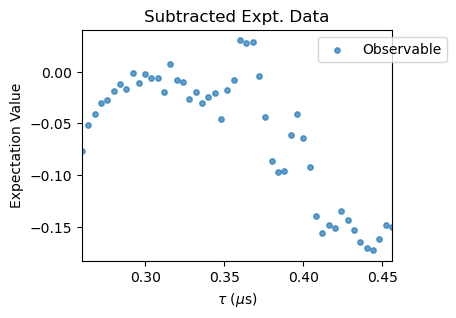
Notice that for large \(N\) pulse errors start to affect the spectra. To correct that, a polynomial baseline corrections needs to be performed with the poly_base_correction method. In succesion, a rescale and offset corrections are applied to the experimental data through the methods rescale_correction and offset_correction.

XYN_exp[10].poly_base_correction(x_start=[0, 32, 42], x_end=[10, 34, -1], poly_order=2)
XYN_exp[11].poly_base_correction(x_start=[0, 31, 39, 47], x_end=[9, 33, 41, -1], poly_order=2)
XYN_exp[12].poly_base_correction(x_start=[0, 31, 38, 46], x_end=[20, 33, 41, -1], poly_order=3)
XYN_exp[13].poly_base_correction(x_start=[0, 30, 38, 45], x_end=[12, 32, 40, 46], poly_order=3)

for idx in range(N.size):
    linear_fit = linregress(XYN_exp[idx].results, XYN_S_sim[idx].results)

    XYN_exp[idx].rescale_correction(linear_fit.slope)
    XYN_exp[idx].offset_correction(-linear_fit.intercept)

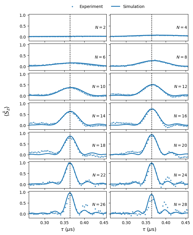
Finally, we plot the comparison between the simulation and experimental data, from which we observe a strong correlation between both.

fig, axs = plt.subplots(int(N.size/2), 2, figsize=(7, 9), sharex=True, sharey=True)

for idx in range(int(N.size/2)):

    axs[idx, 0].scatter(tau, 1-XYN_exp[2*idx].results, c='C0', s=5, alpha=.7, label='Experiment')
    axs[idx, 1].scatter(tau, XYN_exp[2*idx+1].results, c='C0', s=5, alpha=.7)

    axs[idx, 0].plot(tau, 1-XYN_S_sim[2*idx].results, c='C0', lw=2, label='Simulation')
    axs[idx, 1].plot(tau, XYN_S_sim[2*idx+1].results, c='C0', lw=2)

    axs[idx, 0].axvline(tau[26], c='k', lw=1, ls='--')
    axs[idx, 1].axvline(tau[26], c='k', lw=1, ls='--')
    axs[idx, 0].set_xlim(tau[0], tau[-1])

    axs[idx, 0].text(.99, 0.5, f'$N = {N[2*idx]}$', ha='right', va='center', transform=axs[idx, 0].transAxes)
    axs[idx, 1].text(.99, 0.5, f'$N = {N[2*idx+1]}$', ha='right', va='center', transform=axs[idx, 1].transAxes)

fig.text(0, .5, r'$ \langle \tilde{S}_z \rangle $', fontsize=14, rotation=90)
axs[-1, 0].set_xlabel(r'$ \tau $ ($\mu$s)', fontsize=12)
axs[-1, 1].set_xlabel(r'$ \tau $ ($\mu$s)', fontsize=12)
axs[0, 0].legend(frameon=False, loc='upper center', ncols=2, bbox_to_anchor=(1, 1.5))

fig.subplots_adjust(hspace=0.1, wspace=0.05)

3. Nuclear Spin

The simulation of nuclear spin follows a similar structure as the electron spin, except that now the observable and initial state need to be redefined.

system.observable = tensor(qeye(3), jmat(1/2,'z'))
system.rho0 = tensor(fock_dm(3, 1), fock_dm(2,0))

XYN_I_sim = np.empty(N.size, dtype=XY)

for idx in range(N.size):

    # defines the simulation object with the parameters
    XYN_I_sim[idx] = XY(
        free_duration = tau,
        pi_pulse_duration = t_pi,
        system = system,
        h1 = w1*system.MW_h1,
        pulse_params = {'f_pulse': system.MW_freqs[0]},
        M = int(N[idx]/2),
    )

    # runs the simulation and stores the results
    XYN_I_sim[idx].run()

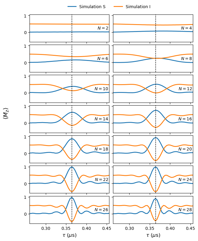
Lastly, we compare the nuclear spin simulations with the electron spin. Where the nuclear spin has a time evolution opposite to the electron, which can be use to form the multi-qubit gates as discussed in the paper.

fig, axs = plt.subplots(int(N.size/2), 2, figsize=(7, 9), sharex=True, sharey=True)

for idx in range(int(N.size/2)):

    axs[idx, 0].plot(tau, 1-XYN_S_sim[2*idx].results, lw=2, label='Simulation S')
    axs[idx, 1].plot(tau, XYN_S_sim[2*idx+1].results,lw=2)

    axs[idx, 0].plot(tau, XYN_I_sim[2*idx].results, lw=2, label='Simulation I')
    axs[idx, 1].plot(tau, XYN_I_sim[2*idx+1].results, lw=2)

    axs[idx, 0].axvline(tau[26], c='k', lw=1, ls='--')
    axs[idx, 1].axvline(tau[26], c='k', lw=1, ls='--')
    axs[idx, 0].set_xlim(tau[0], tau[-1])

    axs[idx, 0].text(.99, 0.5, f'$N = {N[2*idx]}$', ha='right', va='center', transform=axs[idx, 0].transAxes)
    axs[idx, 1].text(.99, 0.5, f'$N = {N[2*idx+1]}$', ha='right', va='center', transform=axs[idx, 1].transAxes)

fig.text(0, .5, r'$ \langle M_z \rangle $', fontsize=14, rotation=90)
axs[-1, 0].set_xlabel(r'$ \tau $ ($\mu$s)', fontsize=12)
axs[-1, 1].set_xlabel(r'$ \tau $ ($\mu$s)', fontsize=12)
axs[0, 0].legend(frameon=False, loc='upper center', ncols=2, bbox_to_anchor=(1, 1.5))

fig.subplots_adjust(hspace=0.1, wspace=0.05)