In this example we study pulsed experiments with P1 centers in diamond coupled with NVs. The physical description of the problem is discussed in detail at
Trofimov, C. Thessalonikios, V. Deinhart, A. Spyrantis, L. Tsunaki, K. Volkova, K. Höflich, and B. Naydenov, Local nanoscale probing of electron spins using NV centers in diamond, arXiv:2507.13295.
[1]:
import numpy as np
from lmfit import Model

from quaccatoo import P1, PMR, Analysis, fit_five_sinc2, Rabi, RabiModel
1. Double Electron-Electron Resonance (DEER)
Since the P1 centers have 4 orientations and 6 observables for the 14N isotope, we need to define a QSys and PulsedSim objects for each.
[2]:
B0 = (3911 - 1827)/2/28.025
w2 = 3 # RF Rabi frequency in MHz
freqs = np.linspace(900, 1200, 500)
sim_1 = np.empty((6,4), dtype=object)
theta = 0
phi = 0

for obs_idx in range(6):
    for rot_idx in range(4):
        qsys = P1(
            B0 = B0,
            rot_index = rot_idx,
            observable = obs_idx,
            N = 14,
            theta = theta,
            phi_r = phi,
            theta_1 = 90 + theta,
            phi_r_1 = phi
        )

        sim_1[obs_idx][rot_idx] = PMR(
            frequencies = freqs, # frequencies to scan in MHz
            pulse_duration = 1/2/w2, # pulse duration
            system = qsys, # P1 system
            h1 = w2*qsys.h1, # control Hamiltonian
        )

        sim_1[obs_idx][rot_idx].run()
The measured signal is composed by all orientations and observables. Thus, we combine all of them by creating another PMR object and inputing the results of the average.
[3]:
avg_deer = PMR(
            frequencies = freqs,
            pulse_duration = 1/2/w2,
            system = qsys,
            h1 = w2*qsys.h1,
        )

avg_deer.results = np.mean(
    [sim_1[obs_idx][rot_idx].results for obs_idx in range(6) for rot_idx in range(4)]
, axis=0)
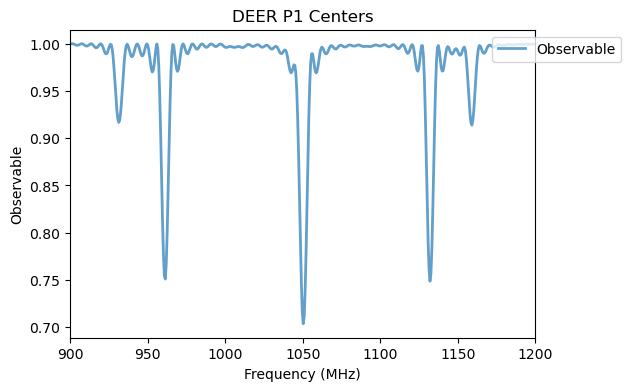
Now we can use the Analysis class to visualize the simulation results.
[4]:
deer_analysis = Analysis(avg_deer)

deer_analysis.plot_results(title='DEER P1 Centers')
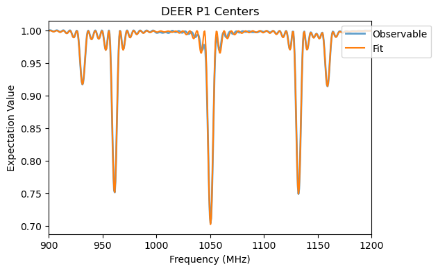
To plot these results we can use five sinc functions, as predefined in QuaCCAToo.
[5]:
fit_guess = {
    'A1': .06,
    'A2': .25,
    'A3': .33,
    'A4': .25,
    'A5': .08,
    'gamma1': 5,
    'gamma2': 5,
    'gamma3': 5,
    'gamma4': 5,
    'gamma5': 5,
    'f01': 930,
    'f02': 960,
    'f03': 1050,
    'f04': 1130,
    'f05': 1160,
    'C': 1,
}

deer_analysis.run_fit(
    fit_model = Model(fit_five_sinc2),
    guess = fit_guess
)

deer_analysis.plot_fit(title='DEER P1 Centers')
deer_analysis.fit_params
[5]:
Fit Result
Model: Model(fit_five_sinc2)
| fitting method | leastsq |
| # function evals | 275 |
| # data points | 500 |
| # variables | 16 |
| chi-square | 0.00381701 |
| reduced chi-square | 7.8864e-06 |
| Akaike info crit. | -5859.44786 |
| Bayesian info crit. | -5792.01413 |
| R-squared | 0.99691184 |
| name | value | standard error | relative error | initial value | min | max | vary |
|---|---|---|---|---|---|---|---|
| A1 | 0.08259495 | 0.00125331 | (1.52%) | 0.06 | -inf | inf | True |
| A2 | 0.24918992 | 0.00124870 | (0.50%) | 0.25 | -inf | inf | True |
| A3 | 0.29728219 | 0.00120064 | (0.40%) | 0.33 | -inf | inf | True |
| A4 | 0.24927147 | 0.00124900 | (0.50%) | 0.25 | -inf | inf | True |
| A5 | 0.08251850 | 0.00124944 | (1.51%) | 0.08 | -inf | inf | True |
| gamma1 | 2.99872240 | 0.03558103 | (1.19%) | 5.0 | -inf | inf | True |
| gamma2 | 3.00389921 | 0.01165909 | (0.39%) | 5.0 | -inf | inf | True |
| gamma3 | 3.25401776 | 0.01017408 | (0.31%) | 5.0 | -inf | inf | True |
| gamma4 | 2.99995964 | 0.01162976 | (0.39%) | 5.0 | -inf | inf | True |
| gamma5 | 3.00267622 | 0.03564813 | (1.19%) | 5.0 | -inf | inf | True |
| f01 | 931.335682 | 0.03672380 | (0.00%) | 930.0 | -inf | inf | True |
| f02 | 961.108542 | 0.01218070 | (0.00%) | 960.0 | -inf | inf | True |
| f03 | 1050.33187 | 0.01062463 | (0.00%) | 1050.0 | -inf | inf | True |
| f04 | 1132.13928 | 0.01217570 | (0.00%) | 1130.0 | -inf | inf | True |
| f05 | 1159.02851 | 0.03678481 | (0.00%) | 1160.0 | -inf | inf | True |
| C | 0.99955597 | 1.4113e-04 | (0.01%) | 1.0 | -inf | inf | True |
| Parameter1 | Parameter 2 | Correlation |
|---|---|---|
| A1 | gamma1 | -0.3773 |
| A5 | gamma5 | -0.3723 |
| A2 | gamma2 | -0.3706 |
| A4 | gamma4 | -0.3697 |
| A3 | gamma3 | -0.3668 |
| A3 | C | +0.1597 |
| A1 | C | +0.1571 |
| A4 | C | +0.1515 |
| A2 | C | +0.1508 |
| A5 | C | +0.1427 |
| gamma5 | C | +0.1107 |
| gamma2 | gamma3 | +0.1028 |
| gamma3 | C | +0.1028 |
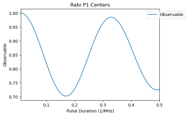
2. Rabi
Now, we keep the frequency of the control field constant in one of the resonances and change the duration of the pulse.
[6]:
B0 = (3911 - 1827)/2/28.025
w2 = 3 # RF Rabi frequency in MHz
freq = 1050.3
sim_2 = np.empty((6,4), dtype=object)
tp = np.linspace(0.01, 0.5, 200) # length of the RF pulse in us

for obs_idx in range(6):
    for rot_idx in range(4):
        qsys = P1(
            B0 = B0,
            rot_index = rot_idx,
            observable = obs_idx,
            N = 14
        )

        sim_2[obs_idx][rot_idx] = Rabi(
            pulse_duration = tp,
            system = qsys, # P1 system
            h1 = w2*qsys.h1, # control Hamiltonian
            pulse_params = {'f_pulse': freq}
        )

        sim_2[obs_idx][rot_idx].run()
Again we combined all simulations for different orientations and observables and plot the data.
[7]:
avg_rabi = Rabi(
            pulse_duration = tp,
            system = qsys, # P1 system
            h1 = w2*qsys.h1, # control Hamiltonian
            pulse_params = {'f_pulse': freq}
        )

avg_rabi.results = np.mean([sim_2[obs_idx][rot_idx].results for obs_idx in range(6) for rot_idx in range(4)], axis=0)

rabi_analysis = Analysis(avg_rabi)
rabi_analysis.plot_results(title='Rabi P1 Centers')
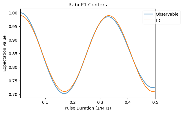
To fit the data em use a fit_rabi function.
[8]:
rabi_analysis.run_fit(
    fit_model = RabiModel()
)

rabi_analysis.plot_fit(title='Rabi P1 Centers')
rabi_analysis.fit_params
[8]:
Fit Result
Model: Model(fit_rabi)
| fitting method | leastsq |
| # function evals | 36 |
| # data points | 200 |
| # variables | 4 |
| chi-square | 0.00844873 |
| reduced chi-square | 4.3106e-05 |
| Akaike info crit. | -2006.41124 |
| Bayesian info crit. | -1993.21797 |
| R-squared | 0.99577518 |
| name | value | standard error | relative error | initial value | min | max | vary |
|---|---|---|---|---|---|---|---|
| amp | 0.13966010 | 6.6056e-04 | (0.47%) | 0.10781286162874283 | -inf | inf | True |
| Tpi | 0.16054186 | 2.9504e-04 | (0.18%) | 0.12311557788944726 | -inf | inf | True |
| phi | 6.08965642 | 0.01031605 | (0.17%) | 4.569589314312426 | -inf | inf | True |
| offset | 0.84952230 | 4.8592e-04 | (0.06%) | 0.8471011167540768 | -inf | inf | True |
| Parameter1 | Parameter 2 | Correlation |
|---|---|---|
| Tpi | phi | +0.8762 |
| amp | Tpi | +0.1796 |
| amp | phi | +0.1627 |
| phi | offset | +0.1508 |