This tutorials reproduces section III.B from:

• 12. Tsunaki, A. Singh, S. Trofimov, & B. Naydenov. (2025). Digital Twin Simulations Toolbox of the Nitrogen-Vacancy Center in Diamond. arXiv:2507.18759 quant-ph. 2507.18759.

The precise detection of weak spins in noisy environments is a central challenge for quantum sensing. At the same time, the coherent control of such magnetic momenta via a central spin is of great interest for quantum simulation and computing. Although they have different goals, both applications can be achieved by dynamical decoupling of the spins from its noisy environment. In the end, the problems is then reduced to precisely modeling the interaction of the central spin (NV’s electron) and the external spin (13C nuclei) under multipulse dynamical decoupling sequences. Following the discussion of the previous section, we first simulate the coherent dynamics of the NV-13.C system in a Hahn echo sequence, as experimentally studied in:

• [1] L. Childress, M. V. G. Dutt, J. M. Taylor, A. S. Zibrov, F. Jelezko, J. Wrachtrup, P. R. Hemmer, and M. D. Lukin, Coherent dynamics of coupled electron and nuclear spin qubits in diamond, Science 314, 281 (2006).

Subsequently, we simulate the detection and control of a weakly coupled 13C by a CPMG sequence, as performed in:

• [2] T. H. Taminiau, J. J. T. Wagenaar, T. van der Sar, F. Jelezko, V. V. Dobrovitski, and R. Hanson, Detection and control of individual nuclear spins using a weakly coupled electron spin, Phys. Rev. Lett. 109, 137602 (2012).

import numpy as np
from quaccatoo import NV, Rabi, square_pulse, Analysis, RabiModel, Hahn, CPMG, save, load
from qutip import jmat, tensor, qeye

1. Electron Spin Echo Envelope Modulations

Once more, we begin the simulation instantiating the NV class with the experimental parameters:

sys1 = NV(
    B0 = 4.2,
    units_B0 = 'mT',
    theta = -45,
    units_angles = 'deg',
    N = 14,
    temp = 300,
    units_temp = 'K'
    )

where we use the theta argument to represent the misalignment of the magnetic field \(\mathbf{B}_0\) with the NV axis \(z\), which by default is 0. In this case then, the magnetic field has a small amplitude of 4.2 mT along the \(\mathbf{z}-\mathbf{x}\) direction. In contrast to Tutorial 3, the nitrogen nuclear spin cannot be neglected, as it slightly shifts the energy levels of the electron spin, thus changing its Larmor frequency and affecting the envelope frequencies of the Hahn echo signal. For that, we set the parameter N to the 14 nitrogen isotope. If the system was otherwise composed with a 15N, additional signals from the nitrogen precession would be observed. However, the same is not true for 14N, due to the quadrupole interaction that fixes the nuclear spin orientation, suppressing its precession. Lastly, for illustration purposes, we set the temperature to 300 K with the temp and units_temp attributes, which calculates the initial state \(\hat{\rho}_0\) from the Boltzmann distribution. If no input is given for temp, as in the other applications, the initial density matrix of the nuclear spin is assumed to be the identity matrix, where for these values of temperature and magnetic field the thermal polarization is minimum.

The coupling Hamiltonian has a hyperfine coupling tensor in units of MHz as

\[\begin{split}\mathbf{A}^c_{hf} = \begin{bmatrix} 5.0 & -6.3 & -2.9 \\ -6.3 & 4.2 & -2.3 \\ -2.9 & -2.3 & 8.2 \end{bmatrix} ,\end{split}\]

representing a weaker coupling compared to Tutorial 3, but still prominent. The representation of \(\hat{H}_2\) and composition with the NV is achieved with:

alpha = np.array([[5, -6.3, -2.9],
                 [-6.3, 4.2, -2.3],
                 [-2.9, -2.3, 8.2]])

H2 = (alpha[0, 0]*tensor(jmat(1, 'x'), qeye(3), jmat(1/2, 'x'))
    + alpha[0, 1]*(tensor(jmat(1, 'x'), qeye(3), jmat(1/2, 'y')) + tensor(jmat(1, 'y'), qeye(3), jmat(1/2, 'x')))
    + alpha[0, 2]*(tensor(jmat(1, 'x'), qeye(3), jmat(1/2, 'z')) + tensor(jmat(1, 'z'), qeye(3), jmat(1/2, 'x')))
    + alpha[1, 1]*tensor(jmat(1, 'y'), qeye(3), jmat(1/2, 'y'))
    + alpha[1, 2]*(tensor(jmat(1, 'y'), qeye(3), jmat(1/2, 'z')) + tensor(jmat(1, 'z'), qeye(3), jmat(1/2, 'y')))
    + alpha[2, 2]*tensor(jmat(1, 'z'), qeye(3), jmat(1/2, 'z'))
    - 10.705e-3*sys1.B0*tensor(qeye(3), qeye(3), np.cos(sys1.theta)*jmat(1/2, 'z') + np.sin(sys1.theta)*jmat(1/2, 'x')) )

sys1.add_spin(H2)

Lastly, the Rabi frequency w1 and the the frequency of the MW pulse excitations w0 are defined as follows:

w1 = 15
w0 = np.sum(sys1.energy_levels[12:])/6 - np.sum(sys1.energy_levels[1:6])/6

Here, the frequency of the MW pulse is calculated by subtracting the average of all six nuclear sublevels at \(m_S=+1\) from the ones in \(m_S=0\). This way, with a short hard MW pulse, the \(\ket{m_S=0} \leftrightarrow \ket{m_S=+1}\) transition is obtained, unconditional to the nuclear states, as opposed to Tutorial 3. To simulate and fit a Rabi experiment, we use:

tp = np.linspace(0,0.15,1000)

rabi_sim = Rabi(
    system = sys1,
    pulse_duration = tp,
    h1 = w1*sys1.MW_h1,
    pulse_params = {'f_pulse':w0},
    pulse_shape = square_pulse
    )

rabi_sim.run()
rabi_analysis = Analysis(rabi_sim)
rabi_analysis.run_fit(
    fit_model = RabiModel()
)
rabi_analysis.plot_fit()
rabi_analysis.fit_params

Fit Result

Model: Model(fit_rabi)

Fit Statistics

fitting method	leastsq
# function evals	31
# data points	1000
# variables	4
chi-square	0.18549649
reduced chi-square	1.8624e-04
Akaike info crit.	-8584.47459
Bayesian info crit.	-8564.84357
R-squared	0.99795307

Parameters

name	value	standard error	relative error	initial value	min	max	vary
amp	0.43347093	6.2333e-04	(0.14%)	0.32039296999027467	-inf	inf	True
Tpi	0.03159355	9.9571e-06	(0.03%)	0.03753753753753754	-inf	inf	True
phi	-0.00398910	0.00281910	(70.67%)	1.1423973285781066	-inf	inf	True
offset	0.54128392	4.3834e-04	(0.08%)	0.5622157246159021	-inf	inf	True

Correlations (unreported values are < 0.100)

Parameter1	Parameter 2	Correlation
Tpi	phi	+0.8672
phi	offset	+0.1107

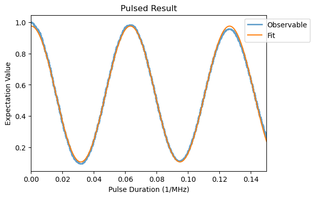
This leads to a \(\pi\)-pulse duration shorter than \(1/(2\omega_1)\), resulting from a hyperfine enhancement effect.

Given the defined system with the experimental parameters, the simplest dynamical decoupling sequence for suppressing the noise from the environment is the Hahn echo technique. The sequence is composed by two free evolutions of duration \(\tau\), with an intermediate \(\pi\)-pulse to the electron spin. In addition, \(\pi/2\)-pulses are included before and after the sequence to drive the electron spin from and to the quantization axis. In NMR, the last projective pulse is not required though, as the measurement is performed perpendicular to the quantization axis. The intermediate \(\pi\)-pulse causes a refocusing of static or slow dephasings, such as those arising from the 14N nuclear spin. This allows the coupled 13C nuclear spin to be probed by the NV.

For performing a Hahn echo simulation in the software component, we use the Hahn class:

tau_hahn = np.linspace(0.04,4,2000)

hahn_sim = Hahn(
    free_duration = tau_hahn,
    pi_pulse_duration = 0.0316,
    system = sys1,
    h1 = w1*sys1.MW_h1,
    pulse_params = {'f_pulse':w0},
    projection_pulse = True,
    time_steps = 1000
    )

hahn_sim.run()
Analysis(hahn_sim).plot_results()

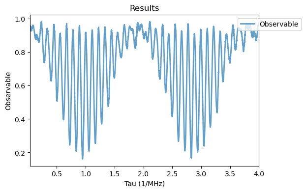
with the same arguments as defined previously. In addition, free_duration is the array containing the \(\tau\) values to be simulated, MW_h1 is the attribute of the sys1 object containing the standard MW control Hamiltonian operator \(\hat{h}_1 = \sqrt{2} \hat{S_x}\), pi_pulse_duration is the duration of the simulated \(\pi\)-pulse, time_steps is the number of discrete time steps used in the simulation in each pulse, and projection_pulse is a Boolean indicating to include a final project \(\pi/2\)-pulse or not, which is set to True by default and will be omitted from now on. It is important to note, however, that the actual pulse separation is the \(\tau\) variable with the duration of the \(\pi\)-pulse subtracted. In most studies, perfect \(\delta\)-pulses are considered and both quantities coincide. Finally, the simulation is executed with the run method, which takes a dictionary containing the options for the parallelization routines. In this case, we include the num_cpusc key as an illustration, which limits the use of the hardware cores for the calculation, in order to avoid over-threading. If the key in the dictionary parameter is not given, the parallelization will run over all of the hardware cores by default.

The results of the Hahn echo simulation show a characteristic Electron Spin Echo Envelope Modulation (ESEEM). The fluorescence observable of the electron spin presents two modulation frequencies. The fast one corresponds to the Larmor frequency of the 13C nuclear spin at the \(m_S=+1\) level, while the slow one corresponds to the one at \(m_S=0\), which is simply given by the gyromagnetic ratio of the nuclear spin \(\gamma^c\) due to the hyperfine coupling being negligible at \(m_S=0\). By measuring these modulation frequencies at different magnetic field \(\mathbf{B}_0\) configurations, the hyperfine interaction matrix can be experimentally reconstructed for arbitrary spins hyperfinely coupled to a central spin.

2. Detection and Control 13C Nuclear spin with CPMG Sequence

The Hahn echo sequence provides a simple mechanism for selective addressing and sensing spins from the environment via the NV center, as demonstrated here. Nonetheless, a robust improvement in the noise filtering can be obtained by repeating the \(\pi\)-pulse and free evolutions several times, known as the CPMG sequence. The periodical reversals of the system’s time evolution cancels out oscillating dephasings and environmental noises from the total evolution, expect for frequencies corresponding to double of the pulse separation \(f_0=1/(2\tau)\) and odd multiples of it. In such manner, weak oscillating magnetic fields from single nuclear spins can be filtered from much stronger backgrounds, even at room temperature. A great improvement compared to superconducting quantum interference device (SQUID) sensing.

For simulating a CPMG sequence of an NV weakly coupled to a lattice 13C, we instantiate the sys2 object with parameters \(B_0=40.1\) mT, \(\theta = 0\) and \(N=14\) as in Ref. [2]. Furthermore the \(\pi\)-pulse duration is set to 10 ns, the frequency of the MW pulse w0 is in resonance with the \(\ket{m_S=0} \leftrightarrow \ket{m_S=-1}\) transition and the hyperfine coupling tensor is

\[\begin{split}\mathbf{A}^c_{hf} = \begin{bmatrix} 0 & 0 & 0.044 \\ 0 & 0 & 0 \\ 0.044 & 0 & 0.032 \end{bmatrix} ,\end{split}\]

in units of MHz. Thus, representing a much weaker coupling than before. To define the system and constants we use:

sys2 = NV(
    B0 = 40.1,
    units_B0 = 'mT',
    N = 14
)

tpi = 0.01
w1 = 1/tpi/2
axz = 0.055 * np.sin(np.pi*54/180)
azz = 0.055 * np.cos(np.pi*54/180)
w02 = 10.705e-3*sys2.B0

H2 = (axz*(tensor(jmat(1, 'x'), qeye(3), jmat(1/2, 'z')) + tensor(jmat(1, 'z'), qeye(3), jmat(1/2, 'x')))
    + azz*tensor(jmat(1, 'z'), qeye(3), jmat(1/2, 'z'))
    - w02*tensor(qeye(3), qeye(3), jmat(1/2, 'z'))
    )
sys2.add_spin(H2)
w0 = np.mean(sys2.energy_levels[6:12]) - np.mean(sys2.energy_levels[1:6])

To run the CPMG simulation with M pulses, we instantiate the CPMG class. Given the high computational cost of the simulation, we execute it in a server with multiple cores using the save method to save the simulations.

sol_opt = {'atol':1e-16, 'rtol':1e-16, 'nsteps':1e8, 'order':30}

tau_cpmg = np.linspace(16.74,16.85,200)

M = [16, 24, 32, 56, 96]

for idx in range(len(M)):

    cpmg_sim = CPMG(
        free_duration = tau_cpmg,
        pi_pulse_duration= 0.00999483,
        system = sys2,
        h1 = w1*sys2.MW_h1,
        pulse_shape=square_pulse,
        pulse_params = {'f_pulse': w0},
        M = M[idx],
        time_steps=1000,
        options={'atol':1e-16, 'rtol':1e-16, 'nsteps': 1e8, 'order':30}
    )

    cpmg_sim.run()
    save(cpmg_sim, f'./sim_data_tutorials/CPMG-{M[idx]}_13C')

The sol_opt variable contains a series of parameters for the ODE solver, which can be passed to the object through the options argument. In this case, the absolute and relative tolerances are decreased, while the number of steps and order are increased, in order to have a more robust solution for such a long pulse sequence.

To retrieve the results we use the load method.

for idx in range(len(M)):
    cpmg_sim = load(f'./sim_data_tutorials/CPMG-{M[idx]}_13C')
    Analysis(cpmg_sim).plot_results()

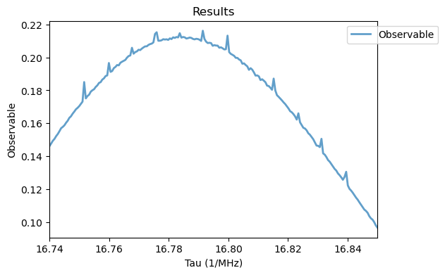
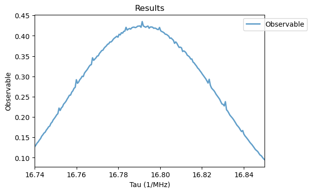
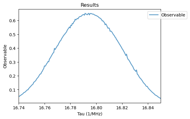
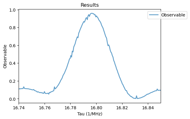
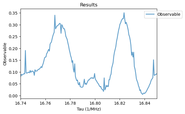
The fluorescence observable shows the 8th order resonance from the weakly coupled 13C spin, displaying oscillations in its intensity as a function of the number of pulses \(M\), due to changes in the filtering function of the multipulse sequence. By keeping a fixed pulse separation value \(\tau\) and changing the number of pulses \(M\), conditional gates can be applied to the nuclear spin exclusively through faster and more precise electron spin pulses. In this way, the NV spin is effectively decoupled from arbitrary oscillating environmental noises, allowing a precise control of the weakly coupled 13C spin. The simulation also presents a small numerical noise, resulting from truncation errors in the ODE solver at such long \(\tau\) values. Both numerical simulations of the Hahn echo and CPMG sequences match the experimental results from Refs. [1, 2], going beyond the semi-analytical model employed there, as it can be used for arbitrary coupling regimes, while considering realistic pulses.