In this example, we consider the simplest two-level system. First, we define the system and plot the energy levels. Following that, a Rabi oscillation is simulated for two different excitation field vectors \(\vec{B}_1(t)\) , with the results being fitted and plotted in the Bloch sphere. Lastly, we simulate a Hahn echo decay for a model collapse operator.
[1]:
import numpy as np
from qutip import sigmax, sigmay, sigmaz, basis

from quaccatoo import QSys, PulsedSim, Analysis, RabiModel, Rabi, Hahn, square_pulse
1. Defining the Spin 1/2 System
We begin defining a general two-level system with a time independent Hamiltonian given by
where \(\omega_0=1\) MHz is the energy difference between the two levels and \(\hat{\sigma}_z\) the Pauli matrix. Although simple, this Hamiltonian can represent a varied number of systems: from spin-1/2 nuclear spins in NMR, to electronic spins in EPR, to superconducting qubits. Let us assume now that the state is initialized in the state \(|0 \rangle\) and that the system has an observable given by the operator \(\sigma_z\).
[2]:
w0 = 1

# create the QSys object with the desired parameters
qsys = QSys(
    H0 = w0/2 * sigmaz(),
    rho0 = basis(2, 0),
    observable = sigmaz(),
    # sets the Hamiltonian units. By default it is considered to be in frequency units.
    units_H0 = 'MHz'
)
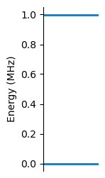
The energy levels are trivial in this simple case. To visualize them we use the plot_energy method from quaccatoo. Note, that in QSys class, the lowest state energy is subtracted from all the eigenenergies to have the lowest level at 0.
[3]:
qsys.plot_energy(figsize=(1,3))
2. Rabi Oscillation
With the quantum system defined, the first measurement to perform is a Rabi oscillation. This is done by applying a resonant pulse to the system with varying length, such that it will drive the system between the two levels causing a period oscillation of the observable expectation value. Let us consider a square cosine pulse of frequency \(\omega_0\) applied on the x-axis of the laboratory frame. The interaction of the pulse with the system is then described in terms of a control Hamiltonian given by
which is then multiplied by the time-dependent pulse function giving \(\hat{H}_1(t)\) . \(\omega_1\) is the Rabi frequency, related to the amplitude of the pulse.
First, let’s consider a rabi frequency 10 times smaller than the resonance frequency \(\omega_1=\omega_0/10\), such that the rotating wave approximation is valid.
[4]:
w1 = w0/10

# create the Rabi object for the qsys and the desired parameters
rabi_sim_1 = Rabi(
    # time array of pulse duration which we want to simulate the experiment
    pulse_duration = np.linspace(0, 40, 1000),
    # we pass the qsys object defined in the previous section
    system = qsys,
    # the Hamiltonian for the interaction with the pulse
    h1 = w1*sigmax(),
    # the pulse shape function we want to use (this line is redundant since square_pulse is the default pulse shape function if not specified)
    pulse_shape = square_pulse,
    # we need to pass the the frequency of the pulse as the resonant frequency of the system
    pulse_params = {'f_pulse': w0},
)

rabi_sim_1.plot_pulses()

To visualize the pulse sequence we can use the plot_pulses method, where we can see the pulse shape and the pulse duration. With the run method the experiment is simulated and the expectation value of the observable is plotted with plot_results.
[5]:
rabi_sim_1.run()

Analysis(rabi_sim_1).plot_results()
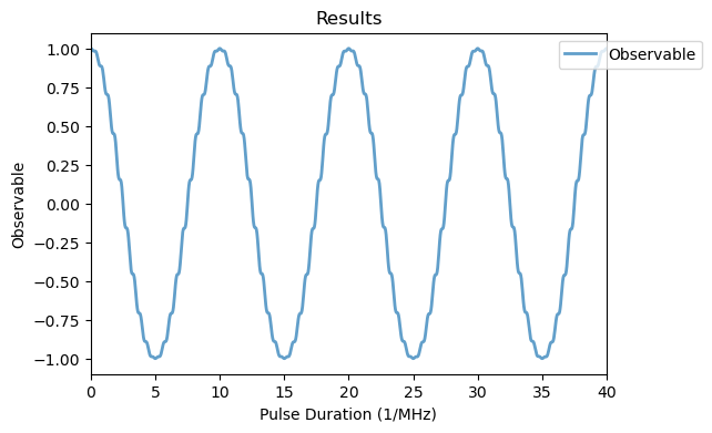
As expected, the expectation value of the operator shows a period oscillation, but with a small modulation related to the rotating wave approximation as we chose \(\omega_0/\omega_1=10\). For larger ratios, this modulation disappears (check yourself!). Now to fit the data we use the Analysis class.
The Analysis instance provides the run_fit method which takes in a fit_model parameter (an lmfit model instance, and optionally also a guess parameter for the initial values). We can then visualize the fit via the plot_fit method. The fit_params attribute contains the detailed fitting report.
[6]:
rabi_analysis_1 = Analysis(rabi_sim_1)

rabi_analysis_1.run_fit(
    # here we use the RabiModel as a target for fitting
    fit_model = RabiModel(),
    )

# plot the results and print the params of the fit
rabi_analysis_1.plot_fit()
rabi_analysis_1.fit_params
[6]:
Fit Result
Model: Model(fit_rabi)
| fitting method | leastsq |
| # function evals | 16 |
| # data points | 1000 |
| # variables | 4 |
| chi-square | 0.62379529 |
| reduced chi-square | 6.2630e-04 |
| Akaike info crit. | -7371.68830 |
| Bayesian info crit. | -7352.05728 |
| R-squared | 0.99875014 |
| name | value | standard error | relative error | initial value | min | max | vary |
|---|---|---|---|---|---|---|---|
| amp | 0.99812524 | 0.00112160 | (0.11%) | 0.9984559815149023 | -inf | inf | True |
| Tpi | 5.00156483 | 7.9437e-04 | (0.02%) | 5.005005005005005 | -inf | inf | True |
| phi | -1.3590e-06 | 0.00228935 | (168452.81%) | 0.0 | -inf | inf | True |
| offset | -6.2572e-04 | 8.0708e-04 | (128.98%) | 6.0341154883046144e-05 | -inf | inf | True |
| Parameter1 | Parameter 2 | Correlation |
|---|---|---|
| Tpi | phi | +0.8718 |
| Tpi | offset | +0.1962 |
| phi | offset | +0.1710 |
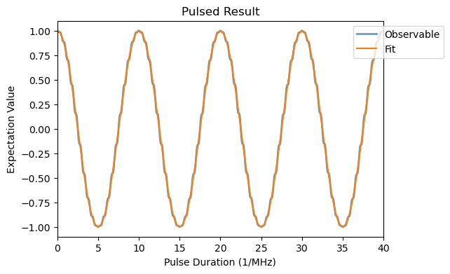
Here, we observe that the fitted value of the \(\pi\)-pulse duration \(t_\pi \cong 5.001\) μs is slightly larger than the expected value of \(1/(2 \omega_1) = 5\) μs. To obtain a more accurate value, we can consider a rotating pulse with two control Hamiltonians \(\hat{\sigma}_x\) and \(\hat{\sigma}_y\), for that we define custom pulse shape for X and Y with a dephasing of \(\pi/2\) as follows.
[7]:
def custom_pulseX(t, **kwargs):
    return np.cos(kwargs['w0']*t)

def custom_pulseY(t, **kwargs):
    return np.cos(kwargs['w0']*t - np.pi/2)

rabi_sim_2 = Rabi(
    pulse_duration = np.linspace(0, 40, 1000),
    system = qsys,
    # the Hamiltonian for the interaction with the pulse now is a list with the two control Hamiltonians for X and Y
    h1 = [w1*sigmax()/2, w1*sigmay()/2],
    # for the pulse_shape we pass a list with the two custom pulse shape functions, as now the custom pulses have no other parameters and pulse_params dictionary is empty
    pulse_shape = [custom_pulseX, custom_pulseY] ,
    pulse_params= {'w0': w0}
)

rabi_sim_2.run()
rabi_analysis_2 = Analysis(rabi_sim_2)

# fit the Rabi oscillations with the run_fit method same as before
rabi_analysis_2.run_fit(
    fit_model = RabiModel(),
    )

rabi_analysis_2.plot_fit()
rabi_analysis_2.fit_params
[7]:
Fit Result
Model: Model(fit_rabi)
| fitting method | leastsq |
| # function evals | 16 |
| # data points | 1000 |
| # variables | 4 |
| chi-square | 2.0777e-08 |
| reduced chi-square | 2.0860e-11 |
| Akaike info crit. | -24589.1886 |
| Bayesian info crit. | -24569.5576 |
| R-squared | 1.00000000 |
| name | value | standard error | relative error | initial value | min | max | vary |
|---|---|---|---|---|---|---|---|
| amp | 0.99999940 | 2.0466e-07 | (0.00%) | 1.0004727285547417 | -inf | inf | True |
| Tpi | 5.00000663 | 1.4466e-07 | (0.00%) | 5.005005005005005 | -inf | inf | True |
| phi | -2.6341e-05 | 4.1706e-07 | (1.58%) | 0.0 | -inf | inf | True |
| offset | -8.1005e-07 | 1.4729e-07 | (18.18%) | 0.0009978644624300977 | -inf | inf | True |
| Parameter1 | Parameter 2 | Correlation |
|---|---|---|
| Tpi | phi | +0.8717 |
| Tpi | offset | +0.1961 |
| phi | offset | +0.1710 |
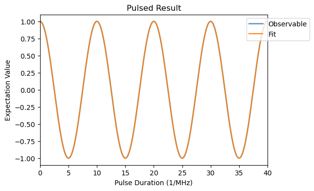
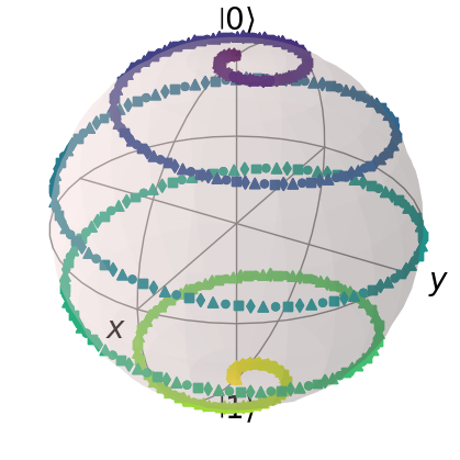
In the rotating frame of reference, this new rotating pulse is fully aligned within the \(x\)-axis. Thus, the modulations have disappeared and the \(t_\pi\) value is closer to the expected value of \(1/(2\omega_1)\). Another useful way to visualize the Rabi oscillation is through the Bloch sphere representation with the plot_bloch method, as shown below. In the rotating frame, the Bloch vector rotates around the \(x\)-axis. However, in the laboratory frame, it rotates in a
spiral.
[8]:
rabi_sim_3 = Rabi(
    # In this case we define a pulse duration array which goes up to a pi-pulse
    pulse_duration = np.linspace(0, 1/2/w1, 500),
    system = qsys,
    h1 = [w1*sigmax()/2, w1*sigmay()/2],
    pulse_shape = [custom_pulseX, custom_pulseY],
    pulse_params= {'w0': w0}
)

rabi_sim_3.run()
rabi_analysis_3 = Analysis(rabi_sim_3)

rabi_analysis_3.plot_bloch()
3. Hahn Echo
Another important quantity in quantum systems is the coherence time \(T_2\), being a measure of how fast a system loses its quantum information, or in other words, how fast it becomes classical. To model the non-unitary process which causes quantum decoherence, we make use of the Lindblad master equation from Qutip. We define as collapse operator
where \(\gamma=0.1\) MHz is rate of decoherence, inversely proportional to \(T_2\). The Hahn echo sequence is then used to measure the coherence time, being composed of two free evolutions with a refocusing \(\pi\)-pulse in between. An initial and final \(\pi/2\)-pulses are also included in order to project the spin the quantization axis.
[9]:
gamma = 0.1

# overwrite the c_ops attribute of the QSys object
qsys.c_ops = gamma * sigmaz()

hahn_sim = Hahn(
    free_duration = np.linspace(5, 25, 30),
    system = qsys,
    pi_pulse_duration= 1/2/w1,
    h1 = w1*sigmax(),
    # include the pi/2 pulse after the second free evolution (this line is redundant since it is the default value)
    projection_pulse=True,
    pulse_shape=square_pulse,
    pulse_params = {'f_pulse': w0}
)

hahn_sim.plot_pulses(tau=10)
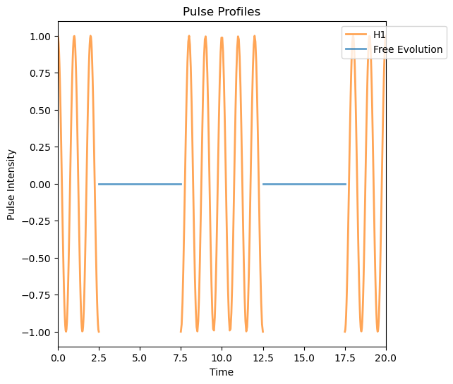
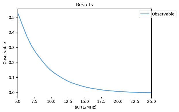
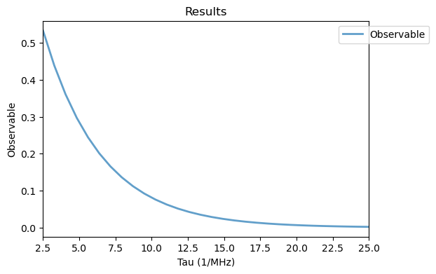
In this case, we can observe the initial and final \(\pi/2\) pulses, the two free evolutions and the middle \(\pi\)-pulse. Finaly, running the experiment leads to an exponential decay of the observable expectation value, known as the Hahn echo decay.
[10]:
hahn_sim.run()
Analysis(hahn_sim).plot_results()
Normally, QuaCCAToo simulates the dynamics of the system by solving the time-evolution under the provided control pulse Hamiltonian \(\hat{H}_1(t)\). However, in many applications, the pulses can be simplified with perfect delta pulses, without temporal length. This has the advantage of being less computationally costly than simulating a time-dependent pulse and to achieve this in QuaCCAToo, the user must set the pi_pulse_duration parameter to 0 and provide an Rx rotational operator
of the pulses.
[11]:
hahn_sim_delta = Hahn(
    free_duration = np.linspace(2.5, 25, 30),
    # here we start from a shorter free evolution time, due to the abscence of the initial pi/2 pulse
    system = qsys,
    pi_pulse_duration= 0,
    Rx = sigmax()
)

hahn_sim_delta.plot_pulses(tau=10)
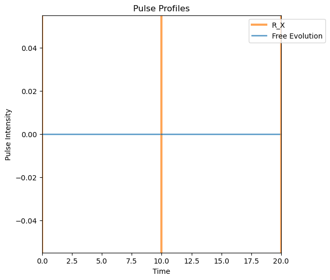
Differently from the previous case, now the pulses appear as vertical line without temporal length. To run the simulation:
[12]:
hahn_sim_delta.run()
Analysis(hahn_sim_delta).plot_results()
Thus, in this case, the consideration of realistic pulses created by a time-dependent Hamiltonian \(\hat{H}_1(t)\) or the assumption of delta pulses, lead to similar results. It’s important to note that the rotation operators are usually defined in the rotating frame, and not the static laboratory frame, which may lead to weird results if the Hamiltonian is not properly defined in the rotating frame.
3.1. Custom sequence
Let’s say now that we want to end the Hahn echo sequence with \(3\pi/2\) pulse instead of \(\pi/2\). This sequence is not predefined in QuaCCAToo, but the user can define it as below. The custom sequence needs to be defined as a python function of a controlled variable, in this case of the free evolution time \(\tau\), and a dictionary with the sequence arguments.
[13]:
def custom_Hahn(tau, **kwargs):

    # calculate pulse separation time !!! pulse separation time is tau - length of a pi-pulse !!!
    ps = tau - kwargs['t_pi']

    # we start initializing the sequence
    seq = PulsedSim(kwargs['qsys'])

    seq.add_pulse(duration=kwargs['t_pi']/2, h1=kwargs['h1'], pulse_shape=kwargs['pulse_shape'], pulse_params = {'f_pulse': kwargs['delta']})
    seq.add_free_evolution(duration=ps)
    seq.add_pulse(duration=kwargs['t_pi'], h1=kwargs['h1'], pulse_shape=kwargs['pulse_shape'], pulse_params = {'f_pulse': kwargs['delta']})
    seq.add_free_evolution(duration=ps)
    seq.add_pulse(duration=3*kwargs['t_pi']/2, h1=kwargs['h1'], pulse_shape=kwargs['pulse_shape'], pulse_params = {'f_pulse': kwargs['delta']})

    return seq.rho

# The sequence arguments are passed through a dictionary
sequence_kwargs = {
    'qsys': qsys,
    'h1': w1*sigmax(),
    'pulse_shape': square_pulse,
    'delta': w0,
    't_pi': 1/2/w1,
    'w1': w1
}

custom_seq = PulsedSim(qsys)
# in this case the run method should be specified with the variable and sequence
custom_seq.run(variable=np.linspace(5, 25, 30), sequence=custom_Hahn, sequence_kwargs=sequence_kwargs)
Analysis(custom_seq).plot_results()
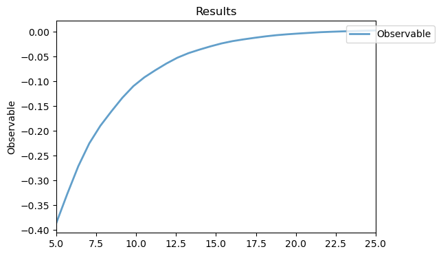
In this case thus, the expectation value start from negatives values then decays to 0 due to the final \(3\pi/2\) pulse.